What is Genome Mapping?
Genome mapping is defined as assigning a specific location to a specific gene on a particular part of chromosomes and then determining the relative distance between two genes present on the chromosomes. The main objective of genomic maps is to help scientists in navigating through the genome and understand the significance of genomic loci and their association with specific conditions. The genomic map is a set of landmarks present on chromosomes; these landmarks include short DNA sequences, regulatory sites for turning genes on and off, and most importantly genes themselves. These genome maps also help scientists to discover new genes.
The significance of genome maps is their application in finding human diseases. The researchers can find disease markers through the genomic maps while studying the affected family, then outlining the inheritance of disease and the association of disease-specific genomic loci over the generations. The loci which appear conserved generation through generation in members having the disease are identified as the genetic marker for the disease. Once such close markers are detected, scientists are able to identify the disease gene location. Thus, with the help of genomic maps, scientists narrow down their research of 3 billion base pair genomes to a few million base pairs.
Besides disease-associated genes, the researchers are also interested in understanding the genome, this allows them to discover novel genes, differentiate between healthy and diseased genes, regulatory networks of genes, and also the role of the non-coding region in gene expression.
There are two types of maps:
Linkage maps or genetic map
Physical maps
The detail of these maps is given in the next section.
Linkage maps/Genetic Maps
A linkage map which is also known as the genetic map is the arrangement of genes and genetic markers along chromosomes based on the frequency with which genes are inherited together. The genes that are close to each other, have more chances to be inherited together. So, just by looking at the pattern of inheritance, we can figure out the genetic distance between genes. Genetic distance in linkage mapping is given by centimorgan or map unit. In modern genetic maps, smaller markers are used which include single nucleotide polymorphism (SNP) between individuals of the same species but the principle remains the same.
The construction of a genetic map is important for genomic studies and also for genetic breeding. Genetic maps have been used for genome assembly, quantitative trait loci (QTL) identification, and comparative genome analysis for many economically important traits. For developing a genetic linkage map, a large number of molecular markers are studied in the related families. Traditional genetic map construction was done by using simple sequence repeats (SSR) and amplified fragment length polymorphism (AFLP) but these lead to a limited amount of QTL identification.
As the next-generation technologies were rapidly developed and bettered, a large number of techniques were applied for genotyping and genome mapping by using SNPs. These techniques include transcriptome sequencing, genome resequencing, restriction site-associated DNA sequencing (RAD-seq), genotyping-by-sequencing (GBS), and specific-locus amplified fragment (SLAF) sequencing. Currently, the popular methodology for the construction of high-density genetic maps is RAD-seq.
With the help of a high-density genetic linkage, we can locate QTLs on the genome and this helps in marker-assisted selection (MAS) which plays quite a crucial role in breeding organisms. QTL allows for studying growth, stress response, disease resistance, and also cold tolerance in many aquatic species.
Physical maps
The physical maps are represented on chromosomes in the form of chromosomal landmarks that show a physical distance between them which is measured in nucleotide bases. Physical maps not only give information about the physical distance between genetic markers but also tells us about the numbers of nucleotides. There are three types of physical maps which are given:
Cytogenetic map: It is obtained by using techniques known as cytogenetic mapping. In this method, mapping is done by using data taken from microscopic analysis of stained parts of chromosomes. It can help us to determine an approximate distance between genetic markers but not an accurate distance.
Radiation hybrid map: This is obtained by using the radiation hybrid method. In order to do mapping, DNA is fragmented by using radiations like X-rays. The size of the segment is adjusted with the help of the amount of incident radiation. The technique helps in overcoming the shortcomings in genetic mapping as it does not depend on the frequency of recombination.
sequence map: This is based on sequence mapping. For mapping, DNA sequence technologies are used to construct a detailed physical map in which the distance between genes is measured in base pairs.
The construction of physical maps has been increased by the creation of many different genomic libraries and cDNA libraries. In order to develop a physical map, a unique genetic site sequence is used which has a known location on chromosomes with a sequencing technique (a sequence-tagged site, or STS). Common STSs include single sequence length polymorphism (SSLP) and expressed sequence tag (EST). SSLPs are found from a set of known genetic markers while EST is determined with cDNA libraries and they give us a link between a genetic and a physical map.
Previously, physical maps were generated by using large DNA fragments which were cloned in vectors like), a bacteriophage P1-derived artificial chromosome (PAC), a yeast artificial chromosome (YAC) or the bacterial artificial chromosome (BAC). A considerable number of clones were created so that all the regions of DNA being mapped must be included. The clones are cut into small fragments with the help of restriction enzymes which are then probed with nucleotide sequences, either bioinformatically or molecularly, to determine a complementary sequence between the inserted DNA fragment and the vector. The clones having overlapping DNA sequences are identified and then a contig map is constructed for each chromosome. Thus, a contig map has overlapping and contiguous DNA fragments. When the contigs are analyzed, the physical distance between markers and genes aisassessed. Besides these, many other methods are present for mapping landmarks on chromosomes or physical mapping.
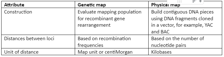
A comparison of the physical map and the genetic map is given by following table 1:
Table 1: Physical map and Genetic map comparison
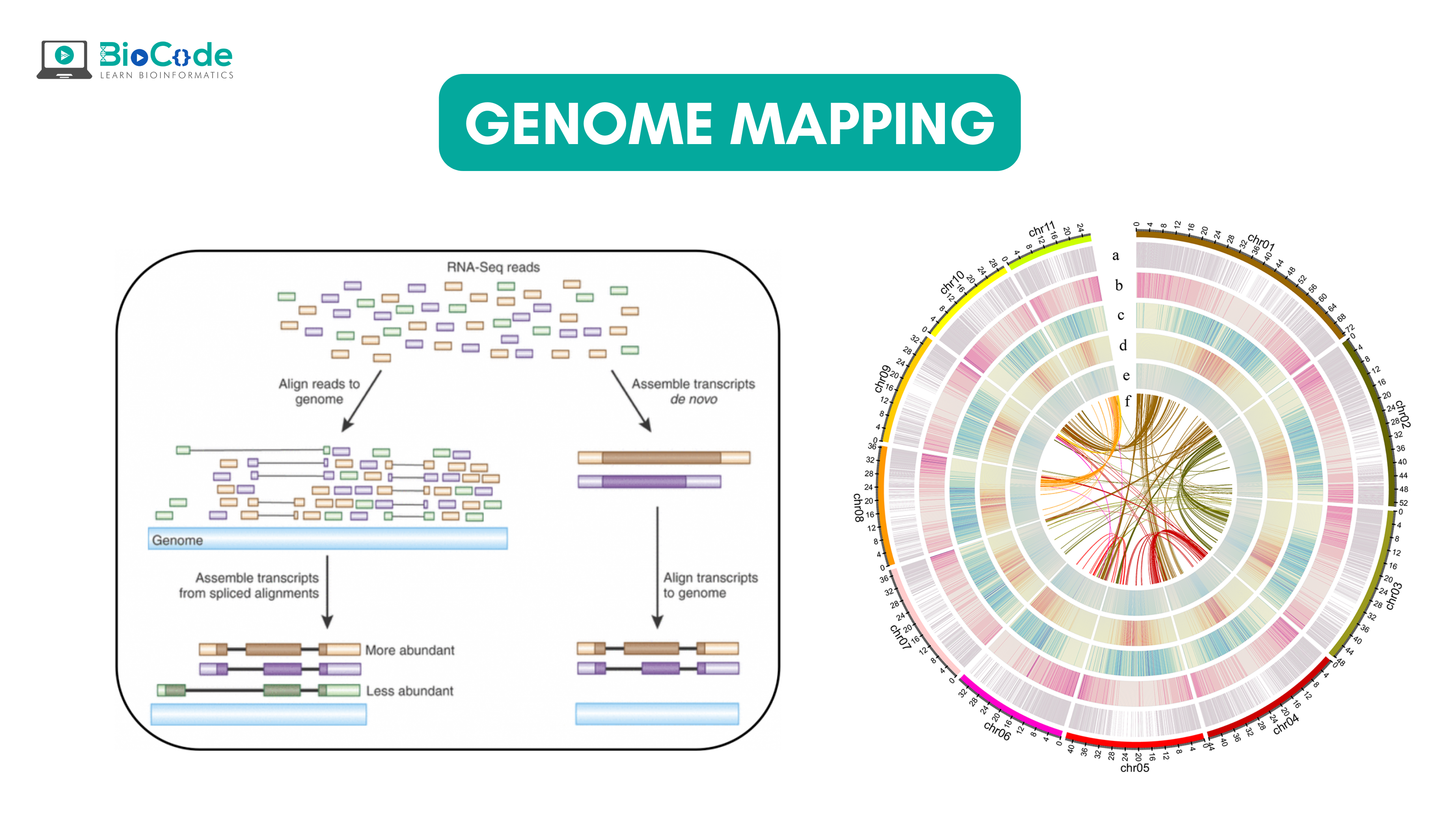
The illustration of genomic map is given by figure 1:
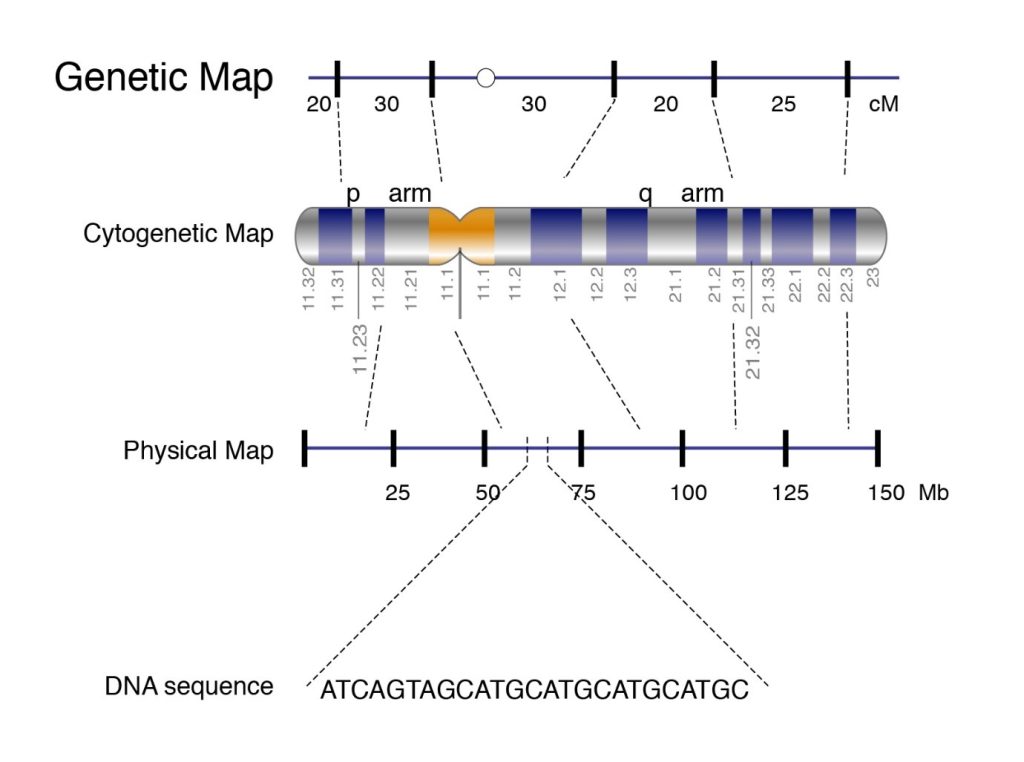
Figure 1: Genome Map
Computational tools for mapping
To do mapping, many computational tools are required. The data for mapping is generated mostly through high-throughput sequencing (HTS). These techniques result in short sequence reads which are then mapped or aligned to a reference genomic sequence. The main challenge is to find the true location of each read efficiently from a large amount of reference genome data while avoiding technical error and taking into account the true genetic variations in the sample.
At present, more than 60 different mapping software are available, most of them developed after 2008. Their development is placed at the same rate as the sequencing technologies. Mappers or alignment tools are designed for the following purposes:
Handle a large amount of data produced from HTS technologies.
Make use of recent development in technologies
Handle protocol development
For instance, alignment tools were developed that use read pairing information after the generation of paired-end library protocols. Also, novel protocols will impact the results by producing certain biases. As the number of tools is increasing, making the right choice is not easy.
Some of the important features of the mappers or alignment software are given by:
Input data
It is the read length that is supported by the mapping tool. There can be mappers of short lead length like that of miRNA data that have short reads ranging between 16-30 bp and the long-read length mappers that can map reads from 1kb to 10 kb. Also, many sequencing platforms produce reads which are quite helpful in detecting alignment errors and also improve specificity and sensitivity in comparison to single-end reads.
As the data produced from HTS is composed of millions of reads so, mappers are mostly executed in a parallel way either in distributed-memory (DM) computers (multiple computers cluster) or/and by shared-memory (SM) computers (present in computers that have shared-memory multi-core processors). As we have to map a large number of reads, the methods are developed that make use of multiple computers or processors for speeding up mapping. Besides these, a cloud-aware mapper is designed that is run in local computer clusters and computer clouds.
Variation and errors
For overcoming or managing the variations and errors, the reads are aligned to a reference genome for approximation. For example, if the study aims to find genomic variations, then the mapping software will allow a small number of errors but sufficient to manage the potential variation. However, when the reads from a different species are aligned to a reference genome or in cases where reads are long, the number of errors allowed increases. The main challenge is to differentiate between a genuine variation or the difference caused due to sequencing error.
To enhance computational efficiency, some of the mapping software limits the number of gaps/mismatches allowed. Also, mappers impose certain constraints on allowed indels. Allowing gaps or indels costs computational efficiency but it is needed sometimes to answer a specific biological question.
Alignments
With the help of mappers, two types of alignments can be done either a global or local alignment. Alignment is crucial to determine the location of interest. A local alignment only takes into account the bases in part of the read and thus is efficient and fast. On the other hand, Global alignment is done end-to-end and it takes time.
Also, there is the case of multimap reads, the cases where reads can align to more than one location and have the same alignment scores. This situation arises due to the repetition of sequences or short lengths of reads. The mappers are specifically designed for multi-reads and are efficient.
The features comparison and important mapping software are given in table 2:
Table 2: Some of the important mapper tools with their feature analysis
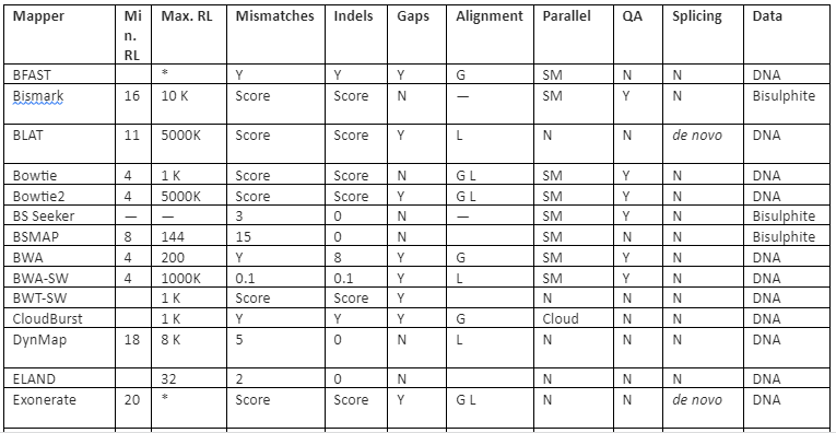
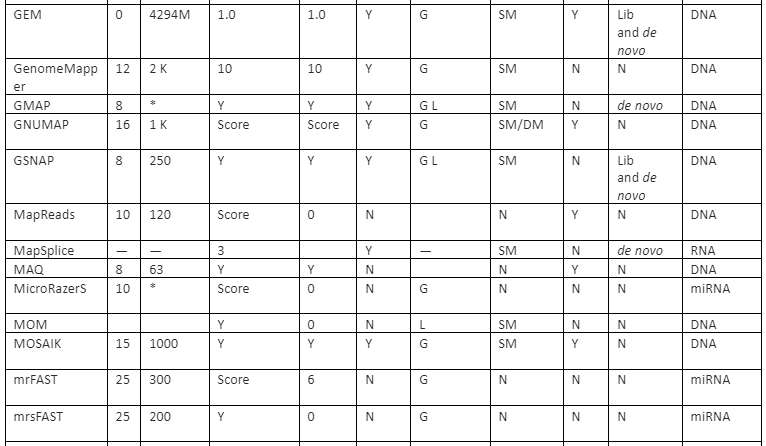
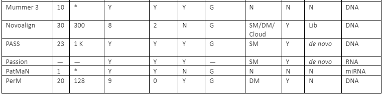
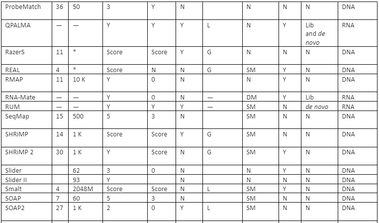
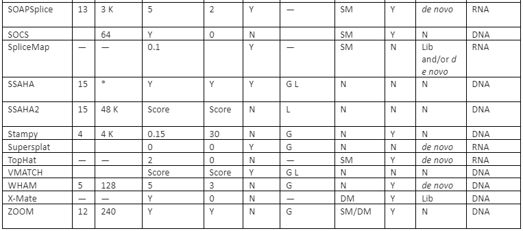
Y=Yes, N=No, RL=Read-lengths, QA=Column Awareness (mapper used read quality information while mapping to reduce errors), Gaps=consecutive indels allowed during analysis, G=Global, L=Local, Parallel column= whether the mapper can be run in parallel and, if yes, how: using an SM or/and a DM computer, *=unknown.
Conclusion
Genome mapping is crucial for understanding genes and gene products. It allows us to identify biomarkers and genes associated with genetic diseases. for mapping, many methodologies and software are present. The choice of method depends upon the type of biological question we are answering. The choice of mapping software is a tough task, as a variety of them are available. It will depend upon the type of analysis needed, input data, and efficiency required.