Single Cell RNA-Seq

What is Single-Cell RNA-Seq (scRNA-seq)?

Single-cell RNA Sequencing technology is a high-throughput method to understand gene expression at the resolution of single cells. Their development has revolutionized the study of transcriptomes as previously the cells were considered homogenous during transcriptomics analysis but in reality, different cells have different properties, so scRNA-Seq provides us with the opportunity to consider each cell individually for gene expression.

History of scRNA-Seq technologies

The pioneer of single-cell sequencing is James Eberwine and his coworkers. They used linear amplification and exponential amplification by in vitro transcription and PCR respectively to expand cDNAs of individual cells. This technology was initially applied to microarray chips and later on adopted by RNA-sequencing technologies to develop scRNA-seq.

The first publication related to the transcriptomic analysis of single-cell was in 2009 in which a Next-generation sequencing platform was used. After this publication, there was a surge of interest from the scientific community to develop high-resolution techniques for studying gene expression at the cellular level depending upon cell heterogeneity. These techniques and technologies enable us to identify rare populations depending upon the differences present in gene expression of individual cells, which otherwise is not possible as the samples are pooled.

ScRNA-Seq Steps

The following steps are involved:

Step One: Isolation of Single cells:

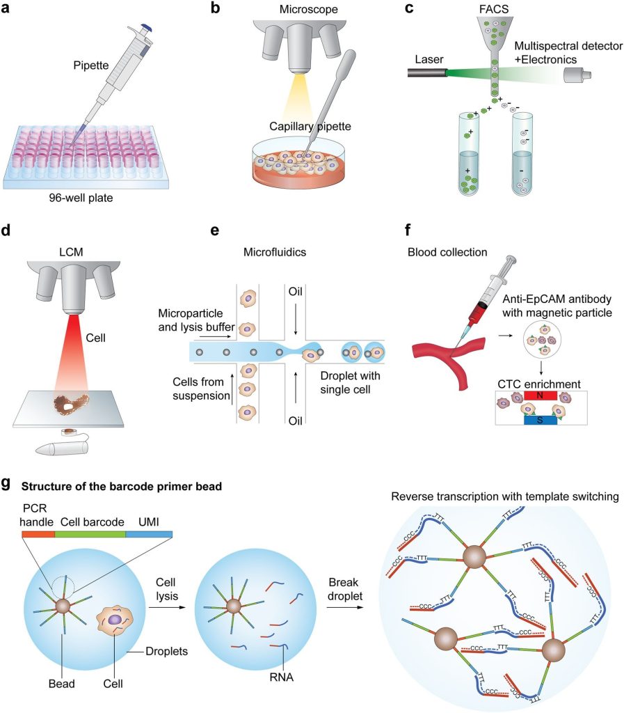
As in scRNA technologies, studies and analysis is done on single cells, so the first step is the isolation of single cells. The main challenge in this regard is the capture efficiency and quality of the cells. At present, many techniques have been adopted to isolate single cells, these include limiting dilution, flow-activated cell sorting (FACS), microfluidics, micromanipulation, and laser capture microdissection (LCM).

In limiting dilution techniques, single-cell isolation is done thorough pipetting. This method is quite inefficient. The Micromanipulation technique is the classical method in which cells are obtained from samples containing a small amount of cell-like uncultivated micro-organisms and embryos. The limitation of the technique is that it is time-consuming, laborious, and low throughput.

FACS is one of the widely used techniques for the isolation of single cells. This method needs a large amount of starting material i.e., >10,000 cells present in suspension. Besides this, LCM is another advanced technique, it isolates cells from solid tissues by employing a computer-aided laser system. Another technique that is becoming popular is microfluidics due to its low use of samples, very precise fluid control, and most importantly low cost of analysis. All the single-cell isolating techniques have advantages and limitations.

Step Two: Preparation scRNA-seq libraries:

To generate scRNA-seq libraries, a comparative analysis is done. The steps involved for library preparation includes:

Cell lysis
First-strand cDNA synthesis through reverse transcription
Second strand synthesis
Amplification of cDNA

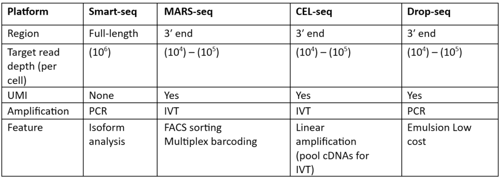
There is a large number of cells present for depth analysis of transcriptomes for library preparation. To make the analysis more effective, efficient and most important cost-effective unique molecular identifiers (UMIs) have been used. These UMIs or barcodes are 4-8 bp sequences that are added in the reverse transcription step. Consider that there are approximately 105–106 molecules of mRNA are present in single cells and it also has more than 10,000 genes expressed. So, we need at least 4bp UMIs. This strategy is allowed us to assign each read to its original cells and also remove PCR bias, thus generating results with high accuracy. With the help of this strategy, not only accuracy but also reproducibility is increased as compared to other approaches. Besides all the advantages, UMIs are mostly tagged at either 5’ or 3’ end, therefore they are not quite useful or suited for isoforms or allele-specific expression. The comparisons of the methods that are used for scRNA-seq library synthesis are given in table 1:

Table 1: Comparison of methods used for preparation scRNA-Seq library

Step Three: Analysis

For analysis of sequence reads many experimental methods are present but there is a great challenge in scRNA-seq due to lack of computational tools which are very limited. Computational tools allow handing off a large number of sequences read data files easily as compared to the experimental methods. Some of the commercially available software tools are 10x Genomics and Fluidigm but overall, there is not a single standard tool developed for this purpose. Some of the computational tools used for the analysis of scRNA-seq data are explained below.

The steps involved in the analysis include:

Pre-processing of data to ensure quality control (QC). For this purpose, Fast QC is used. This tool reviews the quality distribution present across the reads. It also allows the removal of low-quality bases and also adaptors sequences are removed.
Read alignment step for scRNA-seq analysis. The tools available for this purpose are Burrows-Wheeler Aligner (BWA) and STAR. In sequences where UMI are implemented, trimming of the sequence is done before alignment.
Post-alignment summary is then provided by seQC which tells about uniquely mapped reads, coverage patterns related to a specific library, and sequence reads which are mapped to annotated exonic regions. When the transcripts of known sequence and quantity are added for QC and calibration, if a low mapping ratio of endogenous RNA spike in then it is an indication of the low-quality library which is caused due to degradation of RNA or inefficiently lysed cells.
Allocation of sequence reads to exonic, intergenic, or intronic features with the help of transcript annotation in General Transcript Format. The reads which are of high mapping quality and are mapped to exonic loci are considered for producing gene expression matrix, which is given by:

Gene Expression Matrix = N(cells) X M(genes)

Besides these steps, an important distinguishing feature of scRNA-seq data is the zero-inflated counts due to transient gene expression or dropout. To justify this feature, the step of normalization is performed. Normalization diminishes cell-specific bias that can affect downstream applications like the determination of differential gene expression.

In addition to this, there are certain nuisance variables as the sequence read is thought to be directly proportional to the gene-specific expression and cell-specific scaling factors. The estimation difficulty of these nuisance factors allows them to be modeled as fixed factors. These variables can be estimated together with the normalization expression counts but the procedure is quite computationally complex. So, generally, to normalize the raw expression counts, scaling factors are used that estimate by creating a standard across cells. They assume that genes are not differentially expressed. The methods most commonly employed for this purpose include RPKM, FPKM, and TPM (transcript per kilobase million).

RPKM is calculated as (exonic read×109) / (exon length × total mapped read). The difference that exists between RPKM and FPKM is that the FPKM contemplates the read counts in one of the aligned mates only if the paired-end sequencing is performed. The third technique TPM is a modified form of RPKM. In this technique, the sum of all TPMs present in every sample is the same or uniform across samples i.e., exonic read × mean read length×106/exon length × total transcript. These library-sized normalized techniques are quite insufficient for the detection of differentially expressed genes.

In addition to this, two popular methods for between-sample normalization are the trimmed mean of M-values (TMM) method and DESeq. The basis of these frameworks is the idea that counts are dominated by highly variable genes which then skew the relative abundance in expression profile. So, TMM:

Pick up reference samples and consider others as the test samples.
Calculate the M-value of each gene and genes’ log expression ratios present between the test and the reference sample.
Exclude genes with extreme M-values
Set the weighted average M-value of each test sample.

DESeq is almost similar to TMM. However, it calculates the scaling factor as median ratios of each gene’s read count in the particular sample over its geometric mean across all samples. But the limitation in both the approaches is the fact that they both will perform poorly when a large amount of zero counts is present in samples.

Besides these, to avoid stochastic zero counts, the normalization method is developed with pooling expression values which are very robust for differentially expressed genes in the data. In normalization methods, the selection of highly variable genes is sensitive and it can therefore affect the data heterogenic analysis as in most cases highly variable genes are used to reduce the dimensionality before carrying out the clustering analysis.

After the step of normalization, the next step is the estimation of confounding factors. As the observed read counts can be affected by several factors which include biological variables and technical noise. The technical noise is amplified by small starting material. This can be countered by using spike-ins such as ERCC Spike-In Mix from Ambion. The other type of technical variability is caused due to biological variables. To address this issue scLVM method is used.

The schematic of the scRNA analysis pipeline is given in the following figure:

Schematic of the scRNA-seq analysis pipeline. The data of scRNA-seq are noisy with many confounding factors like technical and biological variables. So, after sequencing, (1st step) Alignment and de-duplication are done to quantify an initial gene expression profile matrix. (2nd step) Normalization is done with the help of many statistical methods on raw expression data. (3rd Step) normalized matrix is then put through the main analysis through the clustering of cells for identification of cell subtypes. Cell trajectories can be determined with employment on these data and by detection of differentially expressed genes between clusters.

Currently Available ScRNA-Seq Technologies

Several scRNA-seq technologies have been proposed for carrying out single-cell transcriptomic studies. All the scRNA-seq technologies have the same basic steps. One important difference among these technologies is that the production of sequencing data i.e.,

Production of full length or neatly full-length transcript sequencing data (MATQ-seq and SUPeR-seq)
Sequencing of 3’ end (Seq-Well, Drop-Seq, and SPLit-seq)
Sequencing of 5’ end (STRT seq)

There are also distinct scRNA-Seq protocols that have their appropriate strengths and weaknesses. A study showed that Smart-seq2 can detect a large number of expressed genes in comparison with other scRNA-seq technologies but as per the latest study MATQ-seq can outperform it in the detection of low abundance genes.

In comparison with 3’ and 5’ sequencing, full-length technology of scRNA-seq is more beneficial in allelic expression detection, isoform usage analysis, and RNA editing identification. These advantages are due to their better transcript coverage. Also, full-length coverage techniques can detect lowly expressed transcripts making them more preferable than 3’sequencing methods. It should be noted that the droplet-based techniques like Drop-seq and Chromium can give us large throughput of cells with a low cost of sequencing per cell as compared to the whole- transcript scRNA -seq. therefore, these droplet-based techniques are very useful for obtaining the immense amount of cells to identify cell subpopulations of very complex tissues like tumor samples.

Many scRNA-seq technologies have striking ability to capture both polyA+ and polyA- RNAs such as SUPeR- seq, and MATQ-seq. These protocols are very useful for long noncoding RNAs (lncRNAs) and circular RNAs (circRNAs) sequencing. These lncRNAs and circRNAs are very vital for crucial biological processes and therefore they are biomarkers for cancers. So, these scRNA-seq technologies allow us to explore the gene expression of these dynamic noncoding RNAs and protein-coding RNAs at the single-cell level.

An overview of scRNA-seq is given by following figure 2:

Single Cell RNA-seq overview

Important Applications of Single Cell RNA-seq

Important applications of scRNA-seq are explained below:

Cell type Identification

Cell characterization of human beings is a very complex task. Also, due to cell plasticity, cells can have many potential forms or states throughout development and also in the progression of the disease. But there are very few reliable markers in a given cell type that remain hidden in well-established markers. To reduce the dimensionality, scRNA technology is used which reduces the dimensions through read count normalization. Two types of analysis can be used. Principal component analysis (PCA) and cluster analysis. PCA is the most commonly used analysis that is quite useful in dimensionality reduction. After decreasing the number of dimensions, cell types can be easily identified with accuracy.

Inferring regulatory networks

To visualize gene regulatory networks (GRNs), scRNA-seq can be used. GRNs allow us to comprehend complex cellular processes taking place in living things and also, they can tell us about the interactions taking place in genes and proteins. It must be taken into account, GRN Is not the outcome of a biological study but it is an intermediate bridge that connects genotype with phenotype. Single-cell sequencing allows us to capture thousands of cells that are present in one condition. But it is still difficult due to intracellular heterogeneity. Many methods have been developed which are machine learning-based, co-expression-based, and model-based.

Other applications

Other applications include:

Cell hierarchy reconstruction
Detection of immune cells
Understanding dynamic gene expression

Limitations of scRNA-Seq

These include:

Low capture efficiency and high dropouts
Production of noiser and variable data
Complexity in quality control steps
Need for more computational tools that can be the gold standard