Introduction
Molecular biology, as the terminology describes, is the study of life at molecular level. It is the field of science that is concerned with chemical structures and a variety of biological processes that includes the basic units of life i.e., nucleic acids (DNA and RNA) and proteins. It also helps us to understand the interaction of these essential macromolecules at cellular level.
The recent decade belongs to information technology and computational techniques. Therefore, bioinformatics has also become vital for the molecular biology field. During different types of research in molecular biology like sequencing, a lot of raw data is generated each day and in order to make sense of this data computational techniques are required. Bioinformatics not only organizes genetic data but also helps to make a sense of it. It plays an essential role in analysis of genes, gene expression and regulation. It also allows us to understand many dimensions of evolutionary biology, aids in comparison of genomic data and most importantly it plays a more integrative role by elucidating biological pathways. Besides nucleotide analysis, protein analysis i.e., structure prediction, function and regulation of proteins. Bioinformatics results in 3d simulation of DNA, RNA or protein structures.
In the next section we will discuss the role of bioinformatics in genome analysis, transcriptome analysis and protein analysis.
Genome analysis
The genome of an individual comprises all the genes of an individual’s gene. With the advent of high throughput sequencing technologies and CRISPR-Cas9 system, scientists are able to determine the variations present in coding and non-coding regions. The important outcome of genome analysis is explained below:
Nucleotide Sequencing and analysis
The sequencing is the prerequisite for almost any type of analysis in molecular biology. without knowing and understanding the sequence, nothing can be done. The development of high-throughput sequencing techniques like next-generation sequencing has revolutionaries in the field of molecular biology. It has allowed us to sequence genomes in an efficient and precise way.
The high-throughput sequencing performed with either second generation platforms (Roche/454, Illumina/Solexa, AB/SOLiD, and LIFE/Ion Torrent) or third generation platform Oxford Nanopore, Genia, NABsys, and GnuBio results in generation of huge amount of raw data. In order to understand the output, multiple types of bioinformatics tools and programs are used.
The pipeline of computational analysis of next-generation sequencing has following steps:
Pre-processing of sequences by using FASTQC. This step is crucial to ensure the quality and precision of analysis.
Alignment. It is the process by which the sequence reads are mapped to a reference genome. This is done because in this way short reads are compared with millions of possible positions in the human genome (if reference). This step is computationally complex as the alignment is complicated by the volume of short sequence reads, variations in base quality and also unique versus non-unique mapping. It is also a very critical step because if any errors happen here then they will be carried throughout the analysis.
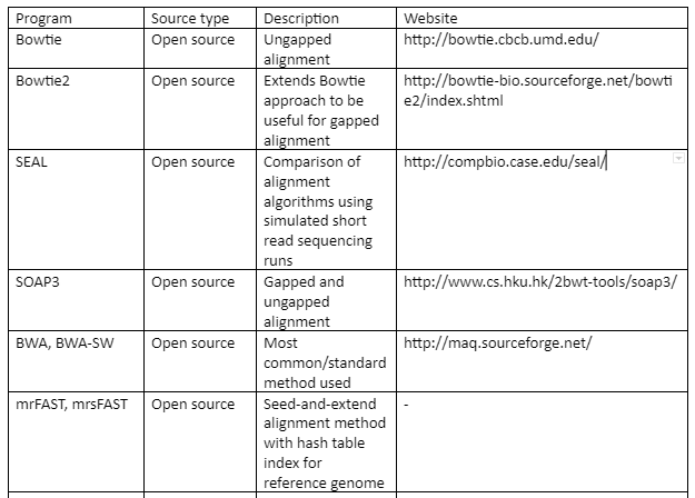
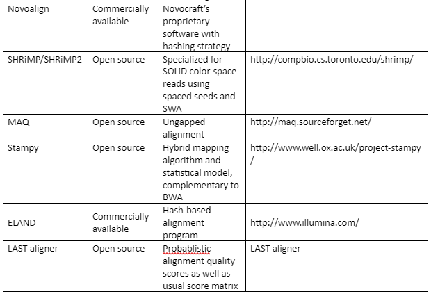
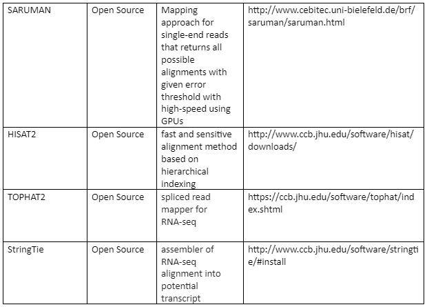
The standard file formats for NGS read alignments are sequence alignment map (SAM) and Binary alignment map (BAM). For alignment many softwares are available as some of them are mentioned in table 1. Most of the alignment algorithms employ an indexing method that allows rapid determination of potential alignment location in the reference genome. The alignment algorithms are employed in aligning short reads to the reference genome is given by table 1:
Table 1: the alignment algorithms for NGS
Variant Calling: After the alignment, the next step is the variant calling. As the alignment of the short reads have already been done, now after the comparison of sample genome with reference genome will help us to identify variants. These variants are responsible for diseases and thus help us to identify the causative agent of a disease at molecular level. We can also identify single nucleotide polymorphism (SNPs) which are related to specific phenotypic expression or are responsible for certain genetic variations.
The standard generic format is Variant call format (VCF) for storing information about sequence variations that includes SNPs, indels, annotations and large structural variants. The challenges faced in variant calling is the identification of “true” variant against the variat due to errors of sequence alignments. The complexity of variant calling is complicated by three important factors:
Presence of indels
Errors in library preparation
Variable quality scores with high levels of errors present at the end of sequence reads.
Therefore, chances of false positive and negative calls are quite imminent. Some of the important variant calling softwares are SOAPsnp, VarScan/VarScan2 and ATLAS 2.
Filtering and Annotation: After variant calling, a list is formed showing thousands of differences present between sample genome and the reference genome. In this step, it is determined which of the variants are involved in the pathological process. At this step, both the filtering, i.e., removing variants that are not present in normal tissue and only fit certain genetic models, and annotation is done.
In addition to filtering, causal variants can be selected on the basis of existing annotation and predicted functional effect. For filtering, many tools have been established that identify genetic variants responsible for disease pathogenesis or phenotypic variance. Some of the tools include Sorting Intolerant from Tolerant (SIFT), PolyPhen/PolyPhen2, VariBench, snpEFF, SeattleSeq, ANNOVAR, Variant Annotation, Analysis and Search Tool (VAAST) and VARIANT.
The overview of NGS analysis is illustrated below:
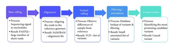
Figure 1: Next Generation sequencing analysis workflow
Gene Prediction
The main aim of gene prediction with the help of computational tools is to locate the protein coding regions. The basic problems faced in gene prediction are of two types: prediction of protein coding regions and prediction of functional site of genes. Many researchers have worked on gene prediction programs and they can be classified into four generations:
The first generation of programs were developed to approximately locate the coding regions present in genomic DNA. The programs most popularly used for this purpose are GRAIL and TestCode. But these programs failed to find the precise location of exons.
The second generation of programs predicted potential exons by combining splice signals and coding region identification. But these programs like Xpound and SORFIND also failed to combine the predicted exon in the form of a complete gene.
The third generation of programs attempted to determine the complete gene structure. For this purpose, a variety of programs were established that includes GeneID, GenLang, GeneParser and FGENEH. But these programs were not quite precise and efficient. Also, all these programs were based on the hypothesis that all the input sequences correspond to a single complete genome.
The fourth-generation programs are developed which are more precise and accurate by using multiple algorithms. These include GENSCAN and AUGUSTUS.
There are two types of methods generally used for prediction of genes i.e.,
Similarity-based Searches: In these approaches a simple similarity search is carried out. It is based on finding gene sequence similarity between expressed sequence tags (ESTs), proteins or the other genomes with input sequence. The principle behind this approach is that the exons as being the functional regions of the genome are more conserved than introns (intergenic regions). After the similarity is determined, it can be used to infer the structure of the gene and also its function. The drawback of this approach is that it only corresponds to a small number of gene sequences and it becomes very difficult to predict the gene structure of a given region.
On similarity searches two important methods are based, these include local alignment and global alignment. The most common local alignment tool is BLAST while for global alignment softwares like PROCRUSTES and GeneWise are used.
In addition to this, heuristic method is applied for pairwise comparison in a software called CSTfinder. The biggest drawback of these techniques is that half of the discovered genes have significant amount of homology with the genes present in database.
Ab initio Prediction: In this second class of approaches, computational identification of genes is to utilize gene structure as a template in order to detect genes. These approaches depend upon only two types of sequence information i.e., signal sensors and content sensors.
Signal sensors are short sequence motifs like branch points, splice sites, start codons and stop codons. The detection of exons depends upon content sensors, which refer to codon usage pattern that are exclusive or unique to a species, and thus allow the discrimination between coding sequencing and surrounding non-coding sequences with the help of statistical detection algorithms.
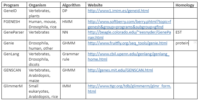
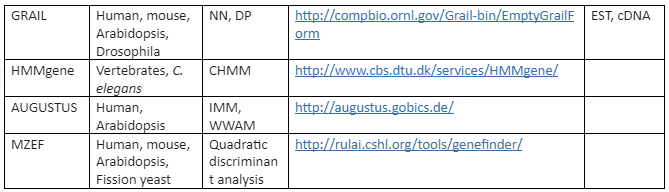
There are a variety of algorithms applied for modeling gene structure like Dynamic programming (DP), linear discriminant analysis (LDA), Linguist method (LM), Neural Network (NN) and Hidden Markov Model (HMM). On these algorithms various tools have been developed for ab initio gene prediction. Some of the most commonly used programs are tabulated in Table 2 while the programs mentioned like Genie, GRAIL and Gene Parser combine similarity searches.
Table 2: ab initio Gene Prediction programs
Genome annotation
After the genome sequencing, genome annotation is done. It is the process by which biological information, especially the functional elements of the genome are identified. The workflow of genome annotation can be given by:
Genome Sequences obtained through high throughput sequencing technologies
Gene Prediction through similarity search or ab initio prediction. At this step for similarity search general databases like NCBI can be used.
Specialized database search for determination of function. The specialized databases include: Domain databases for conserved domains such as Pfam, SMART, and CDD, genome-oriented databases for identification of orthologous relationship, such as COGs for metabolic pathway reconstruction, and refined functional prediction, metabolic databases, such as KEGG
After the function is predicted, further analysis is done.
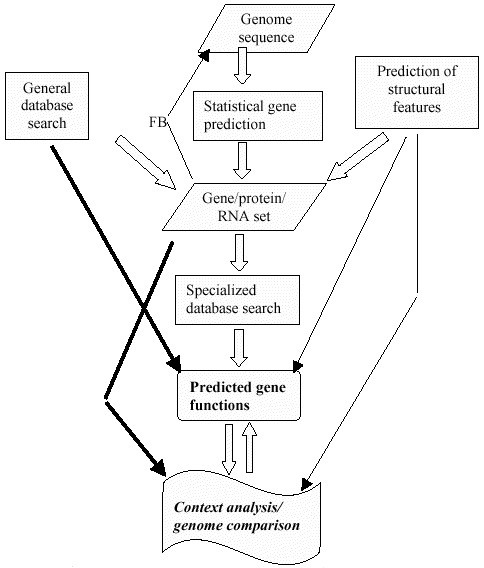
Figure 2: Overview of gene annotation pipeline. Here FB is for feedback.
Now, after the function is determined, the better way to annotate the genome is computationally as it is quite laborious to annotate manually. Some of the automated system for gene annotation are tabulated in Table 3:
Table 3: Automated gene annotation System
In addition to above mentioned tools, there are some of the tools that assist in manual annotation. The example is System for Easy Analysis of Lots of Sequences (SEAL). This tool increases the efficiency of manual annotation.
Transcriptome Analysis
It is the study of transcriptomes, i.e., complete sets of RNA transcript that are made by the genomes under specific situations or promoters in a specific cell, by employing high-throughput methods. Transcription profiling is very useful for studying gene expression which then helps in biomedical research like disease diagnosis, discovery of new biomarkers, risk evaluation of drugs or other environmental chemicals etc. The transcriptome profiling can also be applied to different mutants by loss or gain of function mutations and their association with phenotype.
The early approaches to study transcriptomes were microarray which was replaced by high-throughput sequencing technology like RNA-sequencing. This technique has the ability to detect all types of transcripts in a given sample that includes miRNA, regulatory siRNA and lncRNA. The methodology of RNA-seq includes:
The RNA extraction from sample and then reverse transcription through RT-PCR to make ds-cDNA.
High throughput sequencing is done as per the suitable platform.
Alignment of sequences to the reference genome and identification of transcribed genes
The result will provide the quantitative expression of the transcribed genes.
Then, a detailed analysis is done for the required purpose, like if we want to study gene expression or transcriptional activity of coding or non-coding region, then while analysis, we will choose the softwares which are best suited for this purpose. The analysis of transcriptome data is discussed below.
Analysis of transcriptome data and Related softwares
The most common method for transcriptome data generation is RNA-seq. The workflow of analysis includes following steps:
Pre-processing of raw data: Like any other sequencing, before applying any type of analysis, quality of raw data is ensured. Numerous types of flawed sequence variants can be introduced during the process of library preparation, sequencing and imaging. These erroneous sequences need to be identified and removed. For this the quality control (QC) on raw data is performed. The tools used for this purpose are FastQC and HTQC.
Alignment: The next step is sequence read alignment. In RNA-Seq, two types of reference can be used for alignment, either the genome or transcriptome. The transcriptome consists of all the the transcripts of a given specimen and it has undergone post transcriptional modification i.e., splicing. If transcriptome is used as a reference, then the non-spliced aligners are a proper choice for read mapping. These include Stampy, Mapping and Assembly with Quality (MAQ), and Bowtie. This type of alignment will be limited and it can identify only known exons.
In cases where the genome is used as a reference, splice aligners that permit a wide amount of gaps are used as the read alignments present at exon-exon junctions will split into two fragments. This approach is useful for identification of novel exons. The splice aligners include HISAT2, TopHat, MapSplice, STAR and GSNAP.
RNA-Seq Specific QC: There are many intrinsic biases and limitations like nucleotide composition bias, PCR bias and GC bias that are introduced in RNA-seq data due to low quality or quantity clinical samples. In order to assess these biases, different metrics can be applied like accuracy and bias in gene expression measurement, percentage of rRNA or exonic reads, GC bias, 5’ to 3’ coverage bias and evenness of coverage. The programs used for this purpose include RNA-SeQC and Qualimap 2.
Transcriptome reconstruction: It is the identification of all the transcripts that are expressed in a specimen. In order to accomplish this step, two types of strategies are used which include reference-dependent approach and reference-independent approach. The reference dependent approach is useful when the reference annotation is fully known. This approach is employed in Cufflinks, StringTie and Scripture. In the other cases where the reference genome or transcriptome is not fully known, reference independent approach is applied. It uses a de novo assembly algorithm to directly generate consensus transcripts from the short reads without any reference. This approach is employed in Oases, transABySS and Trinity.
Expression Quantification: Many types of methods have been developed for expression quantification. There are two types of methods based on the target levels. These methods are gene-level quantification and isoform level quantification. The softwares used for gene-level quantification are Alternative expression analysis by sequencing (ALEXA-seq), enhanced read analysis of gene expression (ERANGE), and normalization by expected uniquely mappable area (NEUMA).
On the other hand, isoform-level quantification methods are divided into three categories which depend upon the reference type and requirements of alignment results. The first group of methods need alignment results by using transcriptome as reference e.g., RSEM. The second group of methods need alignment results using whole genome sequences as reference e.g., Cufflinks and StringTie. The last group of methods need alignment free output and it includes Sailfish.
Differential expression analysis: The last step is the differential expression analysis. A gene is said to be differentially expressed if the observed difference or alternation in read count or level of expression between two conditions is statistically significant. In order to have differential gene analysis many softwares have been developed which includes DESeq2, SAMseq, edgeR, Cuffdiff, NOIseq and EBSeq. All these programs employ one or multiple of the available normalization methods to correct bias that can appear between samples, within sample length and GC content.
Although, many tools have been established but according to research there is a large amount of difference that exists between them. Thus, there is not a single optimal tool for differential expression analysis.
Overview of RNA-Seq analysis is illustrated in figure 2:
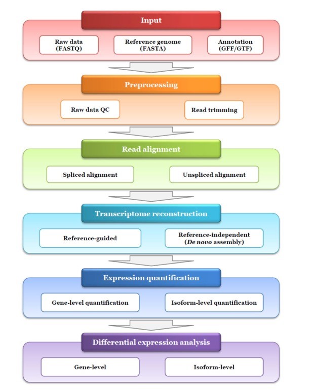
Figure 2: Pipeline of RNA-seq analysis
Protein analysis:
Bioinformatics play an essential role in all the dimensions of protein analysis. This includes sequence analysis, structure analysis and evolution analysis. The brief detail of these aspects is given below:
Sequence analysis:
Protein sequence analysis is done to predict protein structure and function. It is assumed that proteins that have the same amino acid sequences have the same structure. So, in order to understand the protein sequences, protein sequence comparison is done. It also helps us to determine the evolutionary relationships and conserved regions. There are many protein databases which can be employed for protein sequence analysis. A representative example is Prosite databases which have protein sequence patterns and profiles from a large number of families.
Protein Tertiary Structure Prediction
The three-dimensional structure prediction of protein is essential for molecular biology research. Computational techniques have been developed with an aim to devise computer algorithms that have ability to predict three-dimensional structure of protein with input sequence. The main objective behind this aim is to understand protein function at molecular level and also it is quite useful in efficient drug discovery. A major achievement in computer-based native structure prediction programs is CASP.
The computational approaches used for tertiary structure prediction can be categorized into four categories:
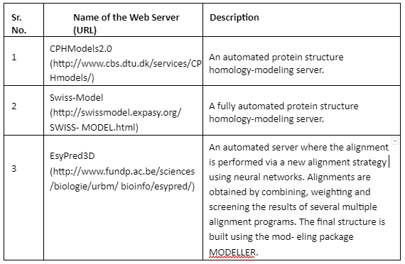
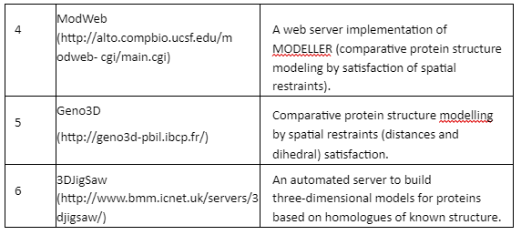
Comparative Modeling or homology modeling: The comparative modeling is based on degree of sequence similarity between proteins. It is based on the assumption that same sequence proteins have similar functions. The accuracy of this technique depends upon the degree of sequence similarity. If the sequence similarity between target and template sequence is more than 50%, then the predictions are considered to be of good quality and accurate. The sequence similarity of 30-50% the quality is moderate while less than 30% means that the prediction has significant errors. The tools employed for comparative modeling are given by Table 4:
Table 4: Tools for comparative modeling
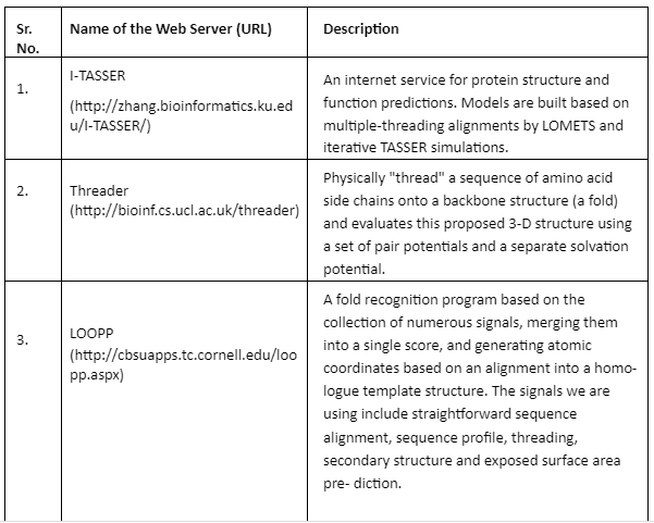
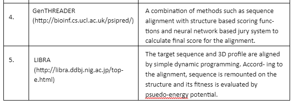
Fold Recognition: In fold recognition and threading methods, a target sequence is fitted to a known structure in the library of folds and then a model is built to evaluate residue-based potentials. This approach joins three different types of pair potentials to account for the fact that different types of scoring function have the ability to assign different target sequences to the same template. After the structurally similar regions are identified in multiple templates then it becomes easy to distinguish between accurate and faulty structures. Some of the important tools are given by Table 5:
Table 5: Fold Recognition tools
First principle method with database information that employs fragment-based recombination methods, hybrid methods that combine multiple sequence comparison, Markov Chain optimization with scoring functions and clustering and the methods that combine information from secondary and selected tertiary structures.
First principle method without database: In this approach, physics based methods without the employment of databases are used to determine native structures and folding processes.
Potential Drug Targets Based On Simple Sequence Properties
Drug analysis is quite efficiently possible with bioinformatics tools. Structure based drug design is playing a very important role in modern drug discovery. The structure information is done through some of the above-mentioned techniques and then mostly with homology modeling potential ligands is screened as a potential drug.
There are numerous drugs that are not successful in the modern drug discovery pipeline and this is due to wrong definition of the target at preclinical states. Recently, a target prediction method has been developed which supports vector machines. In the current methods, physicochemical properties of proteins are taken into account to develop SVM models.
Protein-Protein Interactions
For normal cellular interaction, protein-protein interaction is quite important. Without proper protein interactions, many of the important pathways will be affected. The role and determination of these interactions is a great challenge in molecular biology. Also, there is a protein-protein interaction database that contains the major resources for investigation of biological networks and pathways in cells. The example includes STRING & MPIDB (Microbial protein interaction database).
Conclusion:
It can be concluded in light of the above discussion that bioinformatics plays a key role in bioinformatic research and it has uncovered many important features of the central dogma. But still more research is needed to overcome the limitations.