Introduction
Gene Ontology analysis is used for understanding and interpreting high-throughput data and then developing hypotheses about fundamental biological phenomena. Gene ontology analysis has two main building blocks i.e., ontology and annotation which are evolving rapidly. Ontologies give us a uniform vocabulary for showing domain knowledge. The ontologies are the hierarchical structure of certain concepts defined as the GO terms and their relationship with one another. The Gene annotations are the annotated gene list that is associated with the ontology terms defining those genes. The GO annotation takes into account all the signs and evidence that allow us to associate a gene and a GO term with the help of evidence code. As the amount of available experimental data is increased, the GO and its annotation are evolving continuously. But the annotation of the human genome is still not completed. In addition to this, former GO annotation versions are found to be affected by the biases and confound like annotation bias, in cases where most of the annotations are present for only a few of the well-researched genes. The other bias can be literature bias, in this case, only a small number of articles disproportionally contribute to the experimental annotations. These problems bring challenges in many of its applications like GO enrichment analysis, function prediction of proteins, and gene network analysis.
Composition of Gene Ontology
GO is made up of three types of ontologies which are:
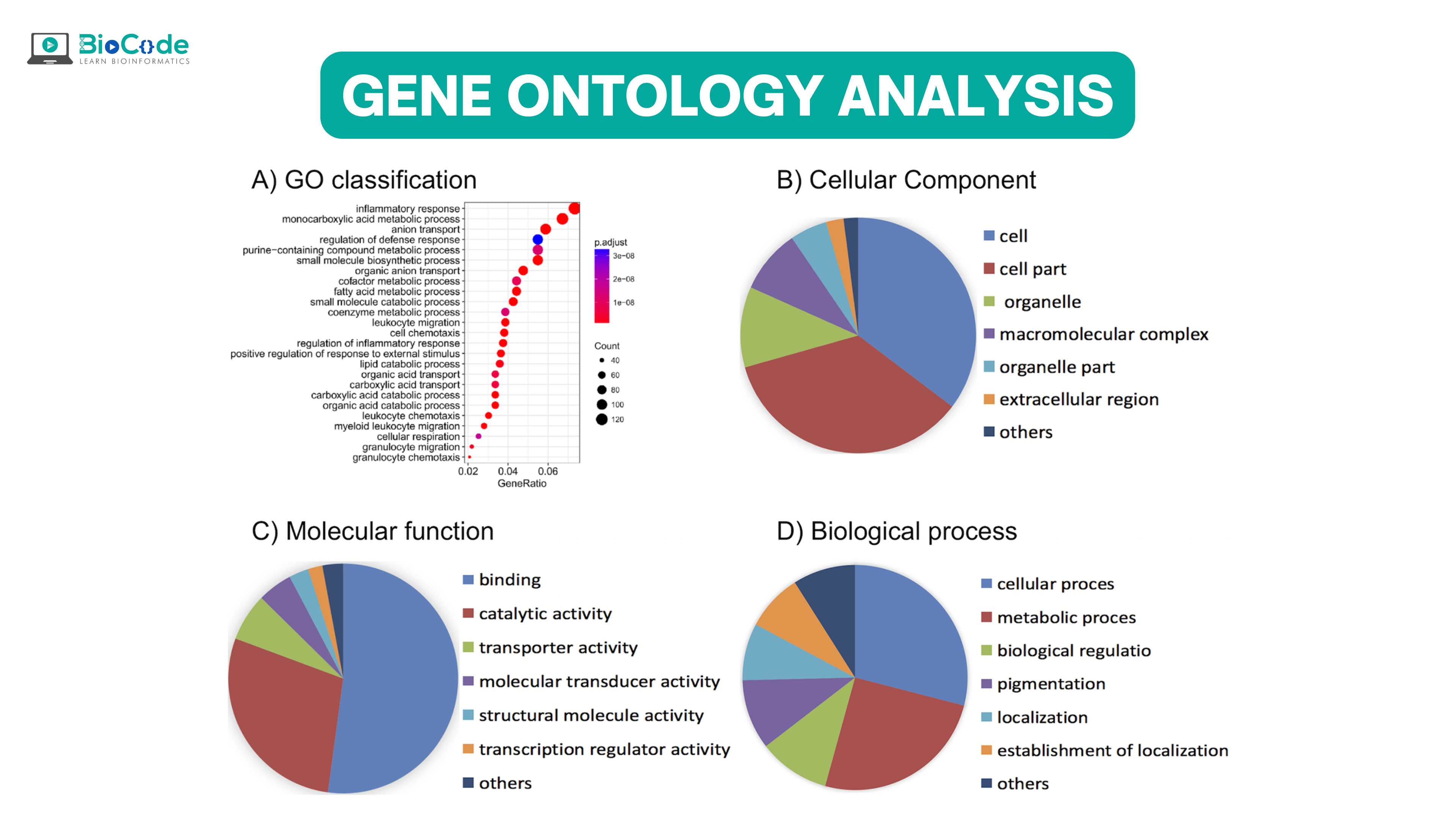
Molecular functional ontology (MFO): It explains the molecular level elemental activities of gene products like catalysis and binding.
Biological process ontology (BPO): It captures the beginning and the end, relevant to the integrated living cell functioning units: cells, tissue, organs, and organism.
cellular component ontology (CCO). It explains the cellular parts and their surrounding (extra-cellular) environment.
Each of these ontologies consists of ontological terms (GO terms) which are then arranged into a hierarchy or directed acyclic graph (DAG). The DAG can be developed by using moderate scripts like Python, R, and Matlab on the ontology file. For defining each of the GO terms, a unique alphanumeric identifier is used and they are viewed at the vertex of the graph, and functions are described by using controlled words. The edge tells us about the relationship i.e., is a, part of and regulated, among GO terms. For instance, if we have GO terms; “GO:0043473”, it will describe pigmentation while “GO:0048066” represents the developmental pigmentation. The two terms are connected by a line that shows the relationship that developmental pigmentation is a subtype of pigmentation.
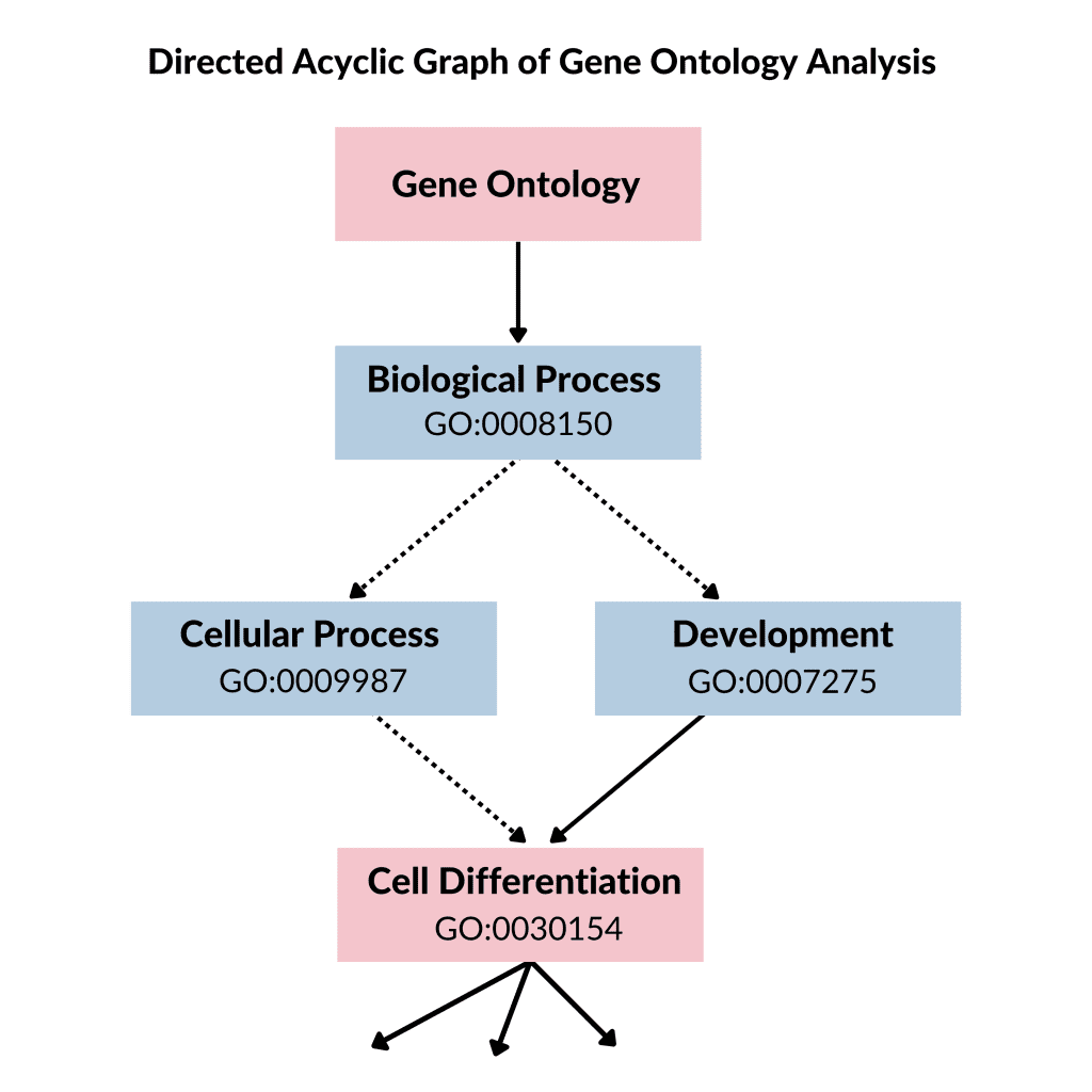
Figure 1: Directed acyclic graph
Another part of GO is the GO annotation. This is the important part of GO as it stores the known functional information about the gene products. There are two types of GO annotation-based function of associated GO term with the gene:
GO positive annotation: It shows that the gene performs the same function as given by the GO term.
GO negative annotation: It shows that the gene product does not carry out the function given by the GO term.
The genes are annotated with GO terms either individually or in groups by the GO consortium. They take the GO terms from the model organisms which are of huge interest among the researchers, for instance, Arabidopsis thaliana, Homo sapiens, Mus musculus, etc. But still, the information and knowledge about the gene product functional taxonomy are immature. Thus, the GO hierarchy and the GO annotations ate continuously updated with new information and saved for future reference. So, it can be said that the knowledge of GO annotation is imbalanced, incomplete, and shallow because some of the species are studied more as compared to others, so different types of species have a different distribution. Also, the number of negative annotations is very small in comparison to positive annotations. This is due to the reluctance of researchers to take it into account as it is not considered useful or publishable and also it can occur due to insufficient experimental conditions.
Workflow of GO analysis by using GOnet
GO analysis is used for the interpretation of high-throughput genomic data and the main purpose of GO analysis is the gene expression analysis of microarray or RNA seq data. In a typical analysis, a gene list is identified as having a differential expression. Then, to understand the significance of modifications in gene expression levels, researchers make use of GO enrichment analysis. in this approach, it is identified whether a GO term related to molecular functions, biological process, or cellular components are over-represented or under-represented in a gene set of interest. Different statistical methods can be used for this purpose and also contain the conventional over-representation of analysis of Functional class scoring or path topology. Here in this section, we will discuss the workflow of GO analysis by using the GOnet tool.
The workflow with GOnet can be divided into two categories i.e., the users’ workflow and the technical workflow.
Users’ Workflow:
In this basic workflow, GOnet receives a list of gene symbols, protein IDs, or protein symbols as input and output in the form of a graph. Many input metrics affect the visualization and structure of the graph. The foremost main choice of the user is the one in which genes are annotated against:
GO terms that are statistically significant and over-represented in the submitted gene list.
A predefined subset (also known as ‘GO slim’)
In the first case, the analysis will be referred to as an ‘enrichment’ analysis, while in the second as an ‘annotation’ analysis.
Input parameters used in GO analysis are:
Gene list. A compulsory input metric that has genes or proteins of interest. At the moment, mouse and human data are supported. The gene list is also followed by a contrast value. It is the value that can be written by any decimal number, such as the long fold-change of gene expression in two conditions. This is only supplied for the enhancement of visualization.
GO namespace. Can be any ‘biological process’, ‘molecular function’, or ‘cellular component’.
Keeping analysis of the three domains separate simplifies the output graph.
Analysis type. Can take the value of ‘enrichment’ or ‘annotation’
Background (in case of ‘enrichment’ analysis only). These contain a baseline gene set against which the signature is analyzed. A user can use as a background:
All annotated genes
Submit a customs
Choose the predefined backgrounds.
In the case where the first option is chosen, the analysis of the signature will be done against all the genes for whom GO annotation knowledge is present. This is the default setting. In the second case, the user can upload a list of genes or proteins for analysis and in the last option ‘predefined background’ allows the analysis of signature against expressed genes having a value of 1TOM in one cell or tissue type as per the availability of expression data in GOnet.
Threshold q-value (only for enrichment analysis). The rejected GO terms will be shown while mitigating the false discovery rate (FDR).
GO subset (for annotation analysis). GO subset annotates against the input entries. The application will generate the relationship of input genes to the GO terms by these metrics.
Output. The results are the default interactive graphs and they are quite useful.
The graphical output allows researchers to do gene and GO term annotation rearrangement so that they can show the discovered functional pattern of classification. User experience will not be the same as it relies on the number of nodes present in graphs and their relationship. If the output has a lot of gene nodes, they can be masked to determine the GO terms only. Alternatively, if the output has too many GO term nodes (like in some cases of enrichment analysis) then varying p-value thresholds can be used to narrow down to the most meaningful enriched groups.
As explained in the above sections, it has become evident that sequencing technologies play an important role in therapeutic diagnosis and treatment. NGS has provided us with a rapid, cost-effective, and real way of decoding the mysteries of diseases like cancer. NGS allows the analysis of inter-tumor and intra-tumor heterogeneity and then identifies biomarkers associated with each type of tumor, helping in diagnosis and drug development. But besides everything, still, a lot of work needs to be done to make NGS more accurate and make computational programs more user-friendly.
Technical Workflow
The overall summary of the steps being applied by the program is illustrated in Fig. 1.
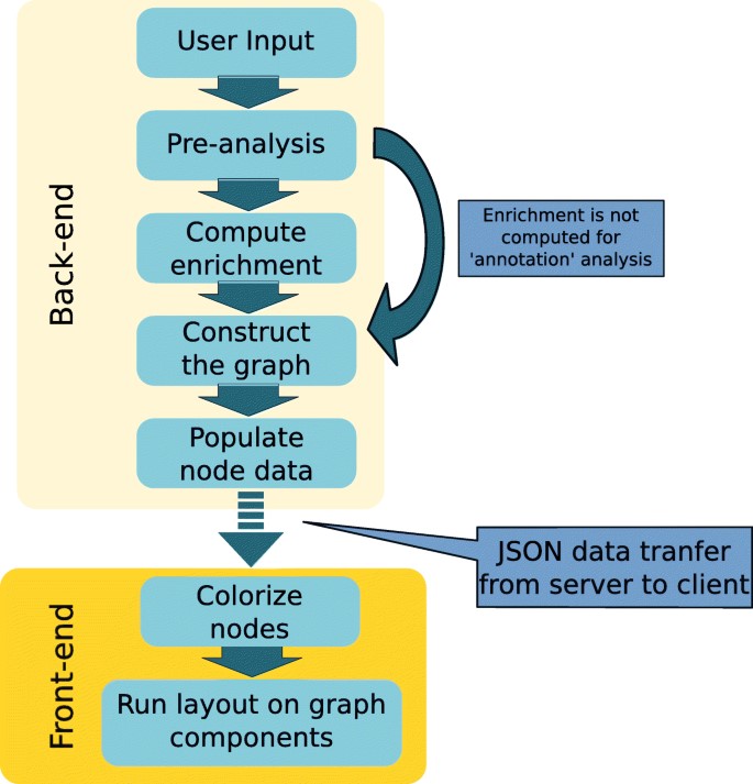
Figure 2: General Outline of GO analysis
The workflow is as follows:
The first step is the pre-analysis. in this step, input checks post submission, and ID conversion is done. The strategy of ID conversion involves the submission of entries by users which are then changed into species-specific primary IDs and then the primary IDs are changed into the IDs. For primary IDs, UniProt IDs and MGI accession IDs are used for human data and mouse data respectively. There will be no conversion into primary ID will take place if the user submits MGI IDs for mice and UniProt IDs for humans. At every step of ID mapping, the programs try to create a one-to-one mapping by choosing the most reliable and relevant IDs. For instance, if we have many UniProt IDs, then those will be selected which belong to the SwissProt subset as they are made through the reliable record. In the scenario where we have duplicated Ensembl IDs, then those IDs are prioritized which are located on the regular chromosomes over the IDs present on alternative loci and the assembly patches. These technicalities allow the program to provide users with the most reliable information and at the same time, it tries to prevent ambiguous interpretation of biological data by using a vast number of cross-references. The final mapped ID is downloaded from the output page. The failed ID entries will also be present in the graph but their associated expression and GO information will not be present.
2nd Step: Compute enrichment. In the second step, Python goenrich package is followed by the computation of enrichment p-values. For every considered GO term, the Fisher exact test p-value is computed. For every GO term, the null hypothesis states that the number of genes in the input list which is annotated with GO term is not overrepresented in the background. The contingency table is given by:
Table 1: Contingency Table
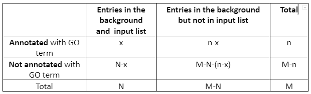
Then p-value is computed as a survival function of the hypergeometric distribution having shape parameters (M, n, N) at point x. After that, all p-values undergo the FDR control protocol. Only those GO categories are taken into the next stage for which the FDR protocol rejects the null hypothesis.
3rd Step: Graph construction: At this step, the program constructs a NetworkX directed graph with the submitted entries and the GO terms. The construction of graph protocol has the following restraints:
The edge will connect the two GO terms if they are directly linked in Gene ontology by the ‘is a’ or ‘part of’ relationship. The direction of the edge is from a more generalized GO term to the specific one.
Genes are linked to the maximum specific GO term available. The direction of edges in the presence of the gene is from GO term to gene.
Nodes that are not related or linked to anything are left as it is and termed as ‘orphan nodes’.
As the GO terms relationship is indicated by the use of ‘is a’ or ‘part of’, it results in the generation of redundancy in the graph. Also, some of the edges are omitted so that if a directed path among any pair of GO term nodes is present in the original graph, then some of the GO terms will be present in a reduced graph. The transitive reduction algorithm is used to make such a reduction graph on the graph from the former step. After that, important data is put in the graph elements.
4th Step: Populate node data. In this step, supplementary information about the elements of the graph is saved as edge attributes or nodes. This includes expression data, IDs (UniProt ID, MGI ID, Ensembl ID), GO references, etc.
Afterward, the graph is converted to cyjs file format and transferred for visualization.
5th Step: Colorize nodes. To differentiate, two different types of color maps are applied to gene nodes and GO terms. The GO terms color intensity indicates the p-value of enrichment. On the other hand expression values are indicated by gene nodes’ colors. During the submission process, these values can be given as contrast values. On the other hand, we can use expression values available from currently supported datasets. The following datasets are supported in the case of human beings:
DICE-DB (http://www.dice-database.org/) data. The dataset covers major blood cell types.
Human Protein Atlas data. Dataset is available at https://www.proteinatlas.org/ and covers major human tissues.
For mouse genes expression data used is taken from the Bgee database.
Run layout. The graph nodes are divided into linked components, after that the user-specific layout is applied to every component. Besides, the orphan nodes are positioned distinctly on the grid.
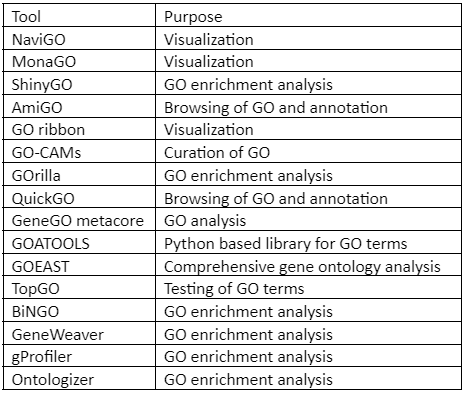
Besides GOnet, Other GO analysis tool includes:
Table 2: Tools for Gene Ontology (GO)analysis and visualization
Conclusion
Gene Ontology has proved itself to be the most dynamic ontology-based resource that offers us tractable and human digestible computational information regarding molecular systems. GO is one of the foremost and pioneer ontologies of the biomedical domain and thus it has pioneered the use of ontologies in computational biology. If GO resources are used smartly and intelligently, then they provide us with the best outcome in the research of biological sciences and medical sciences. GO is one of the better techniques to analyze the pattern in a gene list but sometimes the interpretation of results becomes complicated. No doubt there are many GO enrichment tools that not only carry out the GO enrichment analysis but show us the enriched GO terms from our sets. But these tools mostly have functionality that simplifies the output so that it can be interpreted easily. Thus, the need for a proper visualization tool is required. Also, the selection of gene of interest and background gene set is quite important in GO analysis.